
Vector Search
Visualised
From Zero to Hero in Vector Search
Oct 7 · 2026 · Milvus Meetup, Paris

Why vector search exists...
- 01Maison Lune Wool CoatWrong
- 02Maison Lune Gift CardWrong
- 03Maison Lune Linen Floral MidiMatch
- 04Provence Lavender CandleWrong
- 05Summer Wedding PlannerWrong
Finds the brand, misses the occasion.
- 01Linen Floral Midi · other brandClose
- 02Sage Chiffon Wrap · other brandClose
- 03Maison Lune Linen Floral MidiMatch
- 04Pale Blue Cotton Midi · other brandClose
- 05Blush Silk Slip · other brandClose
Gets the occasion, blurs the brand.
- 01Maison Lune Linen Floral MidiMatch
- 02Maison Lune Sage Wrap DressMatch
- 03Maison Lune Cotton SundressMatch
- 04Maison Lune Pale Blue MidiMatch
- 05Linen Floral Midi · other brandClose
The brand and the occasion.
TakeawayKeyword matches tokens, vectors match meaning. In production you run both: Milvus does BM25 and dense in one query.
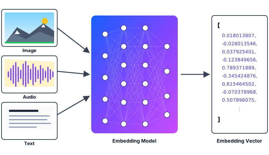
Models turn 'stuff' into numbers
Each model turns its input into an array of numbers - the embedding's position in high-dimensional space. Anywhere from a few hundred to a few thousand Float32 values.
What can we do with them?
RAG
Ground LLMs in your own documents
Agent memory
Recall the right past conversation
Legal analysis
Surface relevant case law
Fraud detection
Spot the needle in a stack of needles
Song matching
Identify a tune from a whistle
Visual search
Find products that look like this photo
Autonomous driving
Detect erratic lane changes
Molecular discovery
Find molecules with similar shape
Cancer screening
Match diagnostic images to known cases
Picturing meaning
Let's build a dress-finder model
What "similar" means
How do you measure similarity in multi-dimensional space?
Exact Search
The naïve approach
Compare the query to every entity in the database. Exact, simple, O(N).
Why flat search doesn't scale
16 dresses, fine. A billion vectors? Not so much. Latency grows linearly and ~all comparisons are waste.
Approximate
nearest neighbour
The trade-off triangle
Every technique trades speed, accuracy & cost.
Recall & Precision: how we measure accuracy
- 01Linen Floral MidiRelevant
- 02Ivory Lace Maxi never wear whiteNot relevant
- 03Sage Chiffon Wrap DressRelevant
- 04Black Wool Sheath not summerNot relevant
- 05Striped Beach Cover-up not a weddingNot relevant
- 06Lavender-Print SundressRelevant
- 07Sequin Cocktail Dress evening, not daytimeNot relevant
- 08Linen Wide-Leg Trousers not a dressNot relevant
- 09Pale Blue Cotton MidiRelevant
- 10Velvet Midi winterNot relevant
- 14Blush Silk Slip MidiRelevant
- 27Terracotta Poplin MaxiRelevant
Of all the good stuff, how much did we find?
Of what we returned, how much was good?
Production notesRecall & precision are measured against exact search, not human judgement.
ThoughtWhat would happen if we filtered to size 38, under €150?
HNSW: navigate a graph
Hierarchical Navigable Small World. Multi-layer graph: top layers have long-range highways, lower layers have local connections. Start at the top, walk greedily closer, drop down a layer, repeat.
IVF: partition the space
IVF clusters the vectors into nlist cells. At query time, only search within the nearest nprobe cells. A true neighbour just over the border of a cell you never open is simply gone.
DiskANN: when RAM runs out
Graph index, engineered for SSD. Minimises random reads, index billions of vectors on ~GBs of RAM.
ANN Benefits
Where ANN lands
Approximate nearest-neighbour algorithms all trade perfection for reduced latency and cost.
The size problem
No matter what algorithm you use, embeddings are big. In RAM or on disk, size matters.
100M chunks and you are holding 1.23 TB before indexing overhead or a single query runs.
Quantisation:
smaller numbers
Scalar quantisation
Round float32 → int8: 4x smaller embeddings, a tiny recall hit & almost no work.
RaBitQ: one bit per dimension
Rotate the space to reduce error, then keep just the sign of each dimension - one bit.
Product quantisation
Scalar quantisation shrinks every number, PQ shrinks the whole vector.
What it costs you (in theory)
Every lost bit risks recall, but the curve is surprisingly forgiving.
Quantisation shifts everything cheaper
Each algorithm can use quantisation to trade accuracy for significantly reduced latency and cost.
Sounds... complex?
All those knobs. Can't the machine work it out?
Trade-offFull control and full responsibility, or one dial and trust the engine.
Dimensionality Reduction:
fewer numbers
PCA: rotate, drop the quiet axes
PCA finds the directions of greatest variance and keeps the top k. Fewer dimensions, full precision.
BenefitKeep one number instead of two and 94% of the variance - linear, fast, deterministic.
DrawbackMaximises for variance, not meaning: structure on a low-variance axis is discarded, and it must be refit when the data shifts.
MRL: one vector, many lengths
The dimensions are ordered by importance, so a prefix is a complete vector.
vs a model not trained for it
MRL tunes the model so the dimensions are ordered by importance. OpenAI's text-embedding-3-large is 3072-D native, but you can ask for any prefix down to 256-D via the dimensions parameter.
BenefitOne model, pick the length per query - short prefix to shortlist fast, full vector to re-rank. Degrades gracefully.
DrawbackOnly works if the model was trained this way - an ordinary embedding survives a light trim, then falls off a cliff once you cut hard (the berry line).
Fewer dimensions, small accuracy hit
Dimensionality reduction nudges any index toward fast and cheap.
Refine: scan cheap, rescore precise
Build time compression and dimensionality reduction both trade accuracy to buy speed and scale. Refinement wins accuracy back at query time.
- Coarse pass - scan
nprobeof the lists using the 1-bit RaBitQ codes. Cheap, and on its own it stops at 0.778. - Refine pass - Milvus keeps SQ8 copies beside the codes and rescores
refine_k × limitcandidates with them. Same candidates, better distances: 0.986. - The last point comes from the coarse pass, not the refine.
nprobe256 to 1024 buys 0.992, at a quarter of the throughput. - Re-ranking is a different axis. A cross-encoder reorders the k you already retrieved. Better ordering, identical recall.
Refinement pulls the other way
Refinement spends a little cost & latency to buy accuracy back.
Filters are tricky
Filtering quietly wrecks your recall
The catchThe harder you filter, the more of the graph you destroy.
There's no single fix - the right technique depends on how much survives the filter.
Three ways out
When retrieval quietly fails
The EXPLAIN you don't get
=# EXPLAIN ANALYZE SELECT * FROM dresses
     WHERE size = 38 AND price < 150;
Index Scan using dresses_size_price_idx
  (cost=0.42..8.44 rows=12)
  (actual time=0.03..0.04 rows=12 loops=1)
  Index Cond: ((size = 38) AND (price < 150))
Execution Time: 0.05 ms
>>> client.search("dresses", data=[q], limit=5,
      filter="size == 38 and price < 150")
- what you got
- #1dress_88120.83
- #2dress_12040.81
- #3dress_09370.80
- #4dress_55210.79
- #5dress_33100.78
- ✕dress_04120.91
- what was there
- #1dress_04120.91
- #2dress_88120.83
- #3dress_12040.81
- #4dress_09370.80
- #5dress_55210.79
The gapSQL fails loudly. Vector search fails silently, so we have to build the instrumentation back ourselves.
Measure what you can't see
Score the index against exact search, on every deploy and every data change.
size == 38 and price < 150
- exact (truth)
- dress_04120.91
- dress_88120.83
- dress_12040.81
- dress_09370.80
- dress_55210.79
- production (ANN)
- dress_88120.83
- dress_12040.81
- dress_09370.80
- dress_55210.79
- dress_33100.78
Average over ~500 real queries, plot it daily.
Recall is a proxy. Users are the truth.
Watch every layerEach layer up is slower and noisier, but closer to what matters. A dip at the bottom is cheap to catch.
Is the index worth it?
Q&A benchmark Recall isn't answer quality
Index recall: does the index match exact search? Answer-presence: is the answer in the top 10?
NQ-Open450 questions10M Wikipedia 2023-11mxbai-embed-large-v111 index configs
Evaluate the model firstThe embedding model and chunking set the ceiling. Measure LGTM@k using exact search before ANN.
Code search benchmark setup Three ways to answer a question
The same question, three ways to feed the model. The search itself is never the expensive part.
No search, no payload. You pay for the answer, and nothing else.
Small results each time. But the whole transcript goes back every turn.
One fat payload of chunks, and a box that bills daily whether you ask or not.
A stronger model grades every answer, without knowing which method was used.
Code benchmark Training data matters
A blind model answered 25 of 40 questions on fastapi, and 0 on a repository published after training cutoff.
fastapi + agentic-hil40 questions eachSonnet 5 agentOpus 5 judgesclaude-context 0.1.15Milvus
Code benchmark Cost per correct answer
Total agent spend over the whole run, divided by the answers the judge marked correct
fastapi + agentic-hil40 questions eachSonnet 5 agentOpus 5 judgesclaude-context 0.1.15Milvus
| Code it knows | Code it has never seen | |
|---|---|---|
| cost | every retrieval arm within ~15% | the index is ~40% cheaper |
| p95 latency | grep 32 s, indexed 46 s | grep 60 s, indexed 39 s |
Memory benchmark Break-even on agentic memory
No memory system vs Milvus memsearch index on a box at $86.07 a month
| Token $ per query | 98k tokens | 392k tokens | 1.2M tokens* |
|---|---|---|---|
| Replay, cache warm | $0.020 | $0.203 | $0.290 |
| Replay, cache cold | $0.393 | $1.569 | $3.839 |
| Index | $0.011 | $0.012 | $0.019 |
| Break-even, cache warm | 334 a day | 15 a day | 10 a day |
| Break-even, cache cold | 7.4 a day | 1.8 a day | 0.7 a day |
Break-even is the box's $2.83 a day divided by the saving per query. Warm uses the measured cache hit rates, 100%, 92% and 97%; cold is a miss on every query, which is what a five-minute cache sees at 15 queries a day. Mean billed cost per query; bars share one scale.
* 1.2M tokens is past the context window: replay keeps 78.5% of the history and answers 47% of questions correctly, against 100% for the index.
synthetic history98k / 392k / 1.2M tokensmemsearch, dense + BM25r8g.large, 16 GiBprices 2026-09-07
Cost Assuming you pay for an index...
I assumed the worst-case - that you provision a VM just for the index
a box of your own
A dedicated r8g.large at $86.07 a month to hold the index. Break-even lands at 10 to 334 queries per day with a warm cache, and under 8 with a cold one.
a box you already run
Milvus Lite or Standalone on your laptop or spare space on an existing box. Same index, same prices, break-even on the first query.
no box at all
Serverless, metered per query with no floor to amortise. Every corpus combined fits into the Zilliz free-forever tier.
Where should it run?
pip install pymilvusNotebooks, prototypes, CI, edge
docker compose upOne box in production
helm install milvusScale-out, with a platform team
pay per request + storageSmall or spiky traffic
provisioned compute, per hourSteady traffic, latency SLAs
storage + compute uptimeHuge dataset, occasional queries
Same engine in every box
In summary
Spend recall on purpose
Every lever in this talk spends recall, buys it back, or checks the balance.
Trade <10% recall for >100× speed, but only if the index is needed.
Up next
So far we've looked at the tech and the numbers, next we'll see what it looks like in production.
19:20 · Criteo
From Product Need to Distributed Vector Search
Mehdi & Peter on why their use case needed a distributed vector database, and the pain points on the way.
20:00 · Gorgias
RAG Design Patterns: Product Indexing at Scale
Mohamed & Othmane on two years of scalability pressure shaping a product index.
Thank you!
simon @ zilliz.com