Vector Search
Visualised

A crash course in vector search

Simon Hearne

solutions architect · zilliz

Why vector search exists...

Keyword search matches intent?

01Comfortable Red Trainers exact phraseMatch
03Comfortable Red Sweater wrong productWrong
04Comfortable Pillow one word matchedWrong
02Personal Trainers Course same word, wrong senseWrong
05Red Wine Glasses one word matchedWrong

Shares words with the query - but not meaning.

Vector search matches intent?

01Comfortable Red TrainersMatch
02Cosy Crimson SneakersMatch
03Snug Burgundy Running ShoesMatch
04Soft Scarlet SneakersMatch
05Cushioned Cherry-Red TrainersMatch

Zero shared words. Same meaning.

Takeaway
Traditional search matches tokens. Vector search matches meaning.

Models turn 'stuff' into numbers

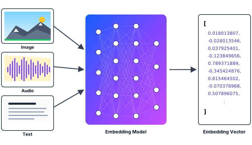
Each model turns its input into an array of numbers - the embedding's position in high-dimensional space. Anywhere from a few hundred to a few thousand Float32 values.

What can we do with them?

📚

RAG

Ground LLMs in your own documents

🧠

Agent memory

Recall the right past conversation

⚖️

Legal analysis

Surface relevant case law

🛡️

Fraud detection

Spot the needle in a stack of needles

🎵

Song matching

Identify a tune from a whistle

🛍️

Visual search

Find products that look like this photo

🚗

Autonomous driving

Detect erratic lane changes

🧬

Molecular discovery

Find molecules with similar shape

🔬

Cancer screening

Match diagnostic images to known cases

Picturing meaning

Let's build a face-finder model

What "similar" means

How do you measure similarity in multi-dimensional space?

Exact Search

The naïve approach

Compare the query to every entity in the database. Exact, simple, O(N).

Why flat search doesn't scale

16 faces, fine. A billion vectors? Not so much. Latency grows linearly and ~all of the comparisons are waste.

The trade-off triangle

Every technique trades speed, accuracy & cost.

Approximate
nearest neighbour

Recall & Precision: how we measure accuracy

Ranked results · vector search 4 of 10 · 6 relevant total

01The Terminator 1984Relevant
02Terminator 2: Judgment Day 1991Relevant
03Terminator 3: Rise of the Machines 2003Relevant
04I, Robot 2004Not relevant
05The Matrix 1999Not relevant
06Westworld 1973Not relevant
07Terminator Salvation 2009Relevant
08Blade Runner 1982Not relevant
09Ex Machina 2014Not relevant
10Looper 2012Not relevant

k = 10 cutoff

14Terminator Genisys 2015Relevant
27Terminator: Dark Fate 2019Relevant

Recall@k

Of all the good stuff, how much did we find?

relevant in top k

total relevant

=

4

6

= 66.7%

Precision@k

Of what we returned, how much was good?

relevant in top k

k

=

4

10

= 40%

Production notes
Recall@k can be calculated against brute force / exact match results

Thought
What would happen if we filtered by release year?

The big idea

~1%recall you give up

→

100-1000×faster, cheaper search

IVF: partition the space

IVF clusters the vectors into nlist cells. At query time, only search within the nearest nprobe cells.

IVF: tuning the knobs

Param	What it does	Bigger means	When it's set	Good default
`nlist`	number of Voronoi cells, set at build	finer cells, slower build, more centroids in RAM	Build	√N
`nprobe`	cells searched per query	higher recall, slower query	Query	8 - 16

Recall too low
Raise nprobe first. If it plateaus, nlist is too high for your data: rebuild with fewer cells.

Too slow
Lower nprobe. Switch IVF_FLAT → IVF_SQ / IVF_PQ to shrink each cell scan.

Memory / build cost
Lower nlist, or use IVF_PQ to compress the vectors inside each cell.

HNSW: navigate a graph

Hierarchical Navigable Small World. Multi-layer graph: top layers have long-range highways, lower layers have local connections. Start at the top, walk greedily closer, drop down a layer, repeat.

HNSW: tuning the knobs

Param	What it does	Bigger means	When it's set	Good default
`M`	edges per node	better recall, more RAM, slower build	Build	16
`efConstruction`	candidate-list width during build	better graph quality, slower build	Build	200
`ef`	candidate-list width per query (≥ k)	higher recall, slower query	Query	64

Recall too low
Raise ef first (no rebuild needed). Still short? Increase M and efConstruction, then rebuild.

Too slow
Lower ef. A higher M lets a lower ef hit the same recall at the cost of higher RAM footprint.

Memory
Lower M, or 2 - 32x savings with quantisation.

DiskANN: when RAM runs out

Graph index, engineered for SSD. Minimises random reads, index billions of vectors on ~GBs of RAM.

DiskANN: tuning the knobs

Param	What it does	Bigger means	When it's set	Good default
`max_degree`	graph out-degree (R)	better recall, larger index, slower build	Build	56
`search_list_size`	build-time beam width (L)	better graph quality, slower build	Build	100
`search_list`	candidate list per query (≥ k)	higher recall, more SSD reads, slower query	Query	100

Recall too low
Raise search_list first. If it plateaus, rebuild with a higher max_degree.

Too slow / spiky p99
Lower search_list. SSD random-read IOPS is the bottleneck - make sure you're on NVMe!

ANN Benefits

Where ANN lands

Approximate nearest-neighbour algorithms all trade perfection for reduced latency and cost.

Sounds... complex?

HNSW, IVF, DiskANN, nlist, nprobe, M, ef, search_list. Can't the machine work it out?

You tune · open-source Milvus / other VectorDB

Pick the index family yourself - IVF, HNSW, DiskANN, GPU…
Set build knobs: nlist, M / efConstruction, graph degree
Set search knobs per query: nprobe, ef - and re-tune as data shifts
Choose quantisation & memory mode by hand

AUTOINDEX decides · managed

You set the metric and performance characteristics
Index type, build params & quantisation derived automatically
One level dial (1 - 10), default targets ~90% recall
Re-optimises per segment as the data moves

Trade-off
Full control and full responsibility, or one dial and trust the engine.

Quantisation:
smaller numbers

Introducing the fingerprint

512 dimensions → a 16×32 grid → hue based on normalised dimension value → a fingerprint for each face.

Similar faces, similar fingerprints

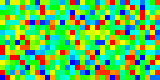
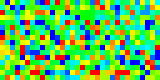
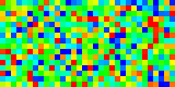
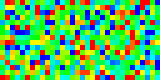
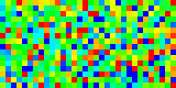
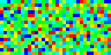
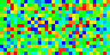
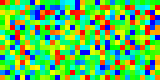
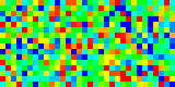
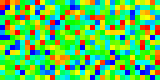
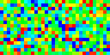
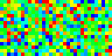
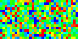
The fingerprint isn't decoration - it is the geometry. Close vectors share a pattern; distant ones don't.

0.43cosine ·
close

vs

−0.35cosine ·
far apart

vs

Scalar quantisation

Indexes make search fast. Quantisation makes vectors small. Round float32 → int8: 4× smaller embeddings, a small recall hit, almost no work.

Cheapest win
No training, no codebook - just rescale each value into a byte. 4× smaller, and most indexes support it out of the box.

How scalar quantisation works

A float32 vector becomes one byte per dimension - step through the moves.

RaBitQ: one bit per dimension

The recent breakthrough: rotate the space, then keep just the sign of each dimension - one bit. The bit-vector preserves angles with a provable error bound, and a cheap correction term sharpens the estimate. Paired with the RaBitQ index in Milvus: up to 32× compression.

Milvus 2.6 · 1M × 768-D
1-bit alone: 32× smaller, recall 0.76. Refine / rescore and recall recovers to 0.95 - at ~4× the throughput of full-precision flat.

How RaBitQ works

Rotate the space, then keep one bit per dimension - step through the moves.

Product quantisation

Scalar quantisation shrinks every number a little. PQ shrinks the whole vector a lot.

Split the 512-D vector into m chunks - say 8 sub-vectors of 64-D.
Cluster each chunk's space with k-means into a small codebook (e.g. 256 centroids).
Replace each chunk with the ID of its nearest centroid - one byte, not 64 floats.
Search by reconstructing approximate distances straight from the codebooks - no decompression.

512 floats collapse to 8 IDs: a barcode.

Warning
PQ leans on a static codebook - learned once, it degrades quietly under model drift.

How PQ works

A 512-D vector becomes eight centroid IDs - step through the four moves.

What it costs you

Every lost bit risks recall, but the curve is surprisingly forgiving.

Quantisation shifts everything cheaper

Each algorithm can use quantisation to trade accuracy for significantly reduced latency and cost.

Dimensionality Reduction:
fewer numbers

PCA: rotate, drop the quiet axes

PCA finds the directions of greatest variance and keeps the top k. Fewer dimensions, full precision.

Benefit
Keep one number instead of two and 94% of the variance - linear, fast, deterministic.

Drawback
Maximises for variance, not meaning: structure on a low-variance axis is discarded, and it must be refit when the data shifts.

Matryoshka: one vector, many lengths

MRL tunes the model so the dimensions are ordered by importance. OpenAI's text-embedding-3-large is 3072-D native, but you can ask for any prefix down to 256-D via the dimensions parameter. The trade-off defers to query time.

Benefit
One model, pick the length per query - short prefix to shortlist fast, full vector to re-rank. Degrades gracefully.

Drawback
Only works if the model was trained this way - truncate an ordinary embedding and recall falls off a cliff (the berry line).

Funnel retrieval with Matryoshka embeddings · milvus.io/blog

How Matryoshka works

The dimensions are ordered by importance, so a prefix is a complete vector - step through the moves.

Fewer dimensions, same precision

Dimensionality reduction nudges any index toward fast and cheap at once.

Refine: search cheap, re-rank precise

Build time compression and dimensionality reduction both trade accuracy to buy speed and scale. Refinement wins accuracy back at query time.

Coarse pass - bulk scan the 1-bit / PQ codes, over-fetch a wider candidate set.
Refine pass - re-rank that shortlist with retained higher-precision vectors.
Return top-k - recall recovers, latency barely moves.

Milvus built-in
Set refine: true at build, tune refine_k at query. Supported on RaBitQ, PQ and SQ indexes.

Superpower
Zilliz uses this technique for indexing external tables, for on-demand lakebase compute.

Refinement pulls the other way

PCA and Matryoshka trade accuracy for speed and cost. Refinement spends a little of both to buy accuracy back - the same triangle, travelled in reverse.

Filters are tricky

Filtering quietly wrecks your recall

Trivial in SQL. On a graph index, the obvious fix quietly backfires 😞

The catch
The harder you filter, the more of the graph you destroy. So there's no single fix - the right technique depends on how much survives the filter.

Three ways out, by selectivity

How much of your data survives the filter decides the strategy.
High selectivity (few pass) → Medium → Low selectivity (most pass)

High · brute force

The filter leaves only a handful of candidates. Skip the graph entirely and compute exact distances over the survivors - cheap because the set is tiny, and 100% recall.

Medium · filter-aware graph

Bake the filter labels into graph construction - the alpha pruning parameter keeps matching nodes reachable. You traverse only valid nodes without fragmenting the index.

Low · post-filter

Almost everything passes, so search the full graph and drop the few non-matches afterward. Over-fetch a little to backfill your k.

What modern engines do
Zilliz watches selectivity per query and picks the strategy automatically - so you stay connected and accurate across the whole range.

When retrieval quietly fails

The EXPLAIN you don't get

SQL / Lucene · fails loudly

EXPLAIN hands you the plan - which index, which scan, what it cost
No match? You get zero rows - an unmistakable signal
You get errors, stack traces, log lines

Vector search · fails silently

You get the k rows you asked for - always
Each carries a rank & score. Nothing else
No plan, no "why", no "were these any good?"

The gap
SQL fails loudly. Vector search fails silently - so we build the instrumentation back ourselves.

Measure what you can't see

You can't eyeball recall. You need a number - and you need it on every deploy.

Build a golden set: freeze a sample of real queries, compute their true neighbours once with exact brute-force - the O(N) scan from the start of this talk. That's your ground truth. Then score the production index against it - recall@k, continuously.

Or let the platform measure it

Maintaining a golden set is work. Zilliz Cloud can compute recall@k for you, per query.

// POST /v2/vectordb/entities/search
{ "data": [[0.12, -0.04, ...]],          // query, embedded
  "limit": 10,                           // k = 10
  "searchParams": { "level": 6, "enableRecallCalculation": true } }

// → response
{ "code": 0,
  "data": [
    { "distance": 0.912, "title": "The Terminator" },      // ✓ relevant
    { "distance": 0.874, "title": "Terminator 3" },        // ✓ relevant
    { "distance": 0.861, "title": "I, Robot" },            // ✗ off-theme
    // … 7 more …
  ],
  "recalls": [0.667] }                   // 4 of 6 true neighbours in top-10

How
It runs your search twice - once at your level, once in a high-precision mode that stands in as ground truth. The brute-force comparison from the last slide, done for you, per query.

Signals of silent degradation

Symptom	Likely cause	Where to look
Recall drops, latency flat	Index params drifted, or the data outgrew them	Raise `nprobe` / `ef` search effort
Recall drops right after a deploy	The embedding model changed	Full reindex - old and new vectors aren't comparable
Fine in tests, wrong in production	Filtering	Pre- vs post-filter; a selective filter wrecked the index
Scores all clustered, none confident	Cross-modal miscalibration	Normalise per modality; add a re-ranker
Recall erodes slowly over weeks	Concept drift - the world moved on	Refresh embeddings; watch the golden set
Memory or cost spiked	Quantisation / index misconfigured	Compression level vs your recall budget

Your agent won't tell you

A database throws an error, an agent won't.

Feed a RAG pipeline or an agent degraded results and nothing crashes. It just gets a bit worse, every time.

The failure never surfaces as a failure.
It surfaces as "the assistant got dumber"

Catch it here
Instrument retrieval itself - recall@k, score spread, filter hit-rate - and watch it before the agent ever consumes the results.

Pro-tip
Use refinement and semantic highlighting to defend against poor results and high token usage.

Strategies that actually work

Determine the correct index for your requirements - HNSW, IVF or DiskANN when RAM runs out. Let AUTOINDEX choose if you'd rather not turn the knobs yourself.
Compress to fit your budget - quantisation (SQ → PQ → RaBitQ) and dimensionality reduction trade recall for memory and speed.
Use query-time levers - experiment with oversampling, refining, semantic highlighting to find the best balance of trade-offs for each use case.
Measure recall@k constantly - version the index alongside the model that built it, and dual-write / A/B at the index level during migrations.
Watch retrieval before the agent consumes it - score spread and filter hit-rate, not just recall@k. And budget for re-embedding from day one; it's not a side-quest.

Thank you!

simon @ zilliz.com